Impedance Control Fundamentals for Bipedal Locomotion

Pure position control is the wrong abstraction for a walking robot. A biped interacting with terrain that isn't perfectly flat doesn't just need to track reference trajectories — it needs to interact compliantly with the surface, absorb impact energy on foot strike, and recover gracefully when the ground is 15mm higher or lower than the model predicted. Impedance control is the framework that makes this possible. But the stiffness-damping parameter space is large, the relationship between parameters and locomotion behavior is nonlinear, and "use impedance control" is not the same as knowing how to parameterize it.
This is a first-principles walkthrough. We'll cover the mechanical model, the difference between impedance and admittance control, how the joint hardware constrains your choices, and what parameter tuning looks like in practice for a bipedal gait cycle.
The Mechanical Model Behind Impedance Control
Impedance control is grounded in the concept of a virtual mass-spring-damper system at the joint output. Instead of commanding the joint to track a position, you command it to behave as if it were a spring and damper with specified stiffness K (Nm/rad) and damping B (Nm·s/rad), attached at the current equilibrium position.
The control law in its simplest single-joint form looks like this:
τ_cmd = K · (θ_eq − θ) + B · (θ̇_eq − θ̇) + τ_gravity
Where θ is the measured joint angle, θ_eq is the desired equilibrium position, θ̇ is the measured joint velocity, and τ_gravity is a feedforward term compensating for gravity loading. The torque command τ_cmd is sent to the motor controller.
This looks like a PD controller with physical units, and it largely is. The difference from classical position control is conceptual rather than mathematical: you're choosing K and B to define a mechanical behavior (how compliant the joint is to external forces) rather than to achieve a tracking bandwidth. A high-stiffness impedance acts like rigid position control; a low-stiffness impedance allows large position deviations in response to small external torques.
For a bipedal robot, this means you can set different impedance parameters during stance phase (stiffer, to maintain posture under body weight) and swing phase (softer, to allow terrain compliance on foot strike without transmitting hard impulses up the kinematic chain). Phase-scheduling of impedance parameters is the primary tool for shaping locomotion behavior.
Impedance vs. Admittance Control: When Each Applies
Impedance control and admittance control are duals of each other. Impedance control takes position error as input and outputs torque. Admittance control takes force (torque) measurement as input and outputs a reference position for an inner position controller to track.
The choice between them depends primarily on the actuator's inherent stiffness. Impedance control works well with backdrivable, low-friction actuators because the torque commands map directly to joint motion — the joint follows the commanded torque without fighting high gear friction. If your joint is stiff and poorly backdrivable (high-ratio planetary gearbox with significant Coulomb friction), impedance control produces jerky, intermittent motion because small torque commands can't overcome the static friction floor.
Admittance control, by contrast, is better suited to stiff actuators. You measure the external force, compute a desired small position correction, and command the inner position loop to track it. The position loop overcomes the friction directly. The downside: admittance control requires a high-bandwidth force sensor at the joint output, and the inner position loop must be fast enough to execute the admittance commands without phase lag.
For a backdrivable strain-wave joint with embedded torque sensing — the hardware configuration we design around — impedance control is the natural choice. The actuator is physically capable of responding to low-level torque commands, and the torque sensor provides the feedback needed to close the loop accurately.
Hardware Requirements That Actually Constrain the Controller
Impedance control theory doesn't talk much about hardware limits, which is where most real implementations run into trouble. There are four hardware properties that directly constrain what you can achieve with an impedance controller on a physical joint:
- Torque sensor bandwidth: The impedance loop needs the torque measurement to be current. A sensor with a 1kHz SPI readout supports 500Hz control bandwidth; slower than that and the damping term (which is velocity-dependent) produces phase lag that destabilizes high-B settings. Sub-millisecond sensor latency is a real requirement, not a marketing spec.
- Motor current loop bandwidth: The motor driver must execute torque commands faster than the impedance loop update rate. If the impedance loop runs at 1kHz but the current loop has a 5ms settling time, the effective impedance bandwidth is limited to the current loop — around 200Hz in that example.
- Backdrive threshold: You cannot implement virtual compliance below the passive friction floor of the gearbox. If the joint requires 8 Nm to backdrive against friction, then commanding K = 0 (zero stiffness) still yields a joint that feels like an 8 Nm spring to any external disturbance smaller than 8 Nm. This is the fundamental floor impedance control cannot cross without active friction compensation.
- Transmission compliance: Strain-wave gearboxes have finite torsional stiffness (typically 2,000–4,000 Nm/rad). This creates a resonant mode between the motor inertia and the output load. If K is set above this natural stiffness, the impedance loop attempts to be stiffer than the transmission allows, which excites the resonance. K_max for a stable impedance controller is typically 0.7–0.9× the transmission stiffness.
Parameterizing Stiffness and Damping for a Bipedal Gait Cycle
Gait cycle impedance scheduling involves at minimum two regimes per leg: stance and swing. In practice, many teams use three or four sub-phases within stance (early contact, mid-stance, push-off, late swing). Here's the general framework we use for ankle and knee parameterization.
During early contact (foot strike to 10% of gait cycle), ankle K should be low — in the range of 200–400 Nm/rad — to allow the foot to conform to ground angle and absorb impact energy. B should be moderate to provide damping without actively resisting the downward rotation. If K is too high here, the impact impulse transmits directly up the leg as a rigid-body collision.
During mid-stance (10–60% of gait cycle), both K and B can increase significantly — ankle K values of 800–1,500 Nm/rad are typical for a ~70kg robot, reflecting the stiffness needed to support body weight through the ankle without large positional drift. This is the phase where the joint functions most like a stiff spring.
Push-off (60–75% of gait cycle) benefits from a transition to explicit torque feedforward — the impedance framework can be held with a non-zero equilibrium torque component to add the propulsive push without waiting for position error to accumulate.
During swing (75–100%), both K and B drop sharply. The foot is in the air; trajectory tracking is lower priority than compliance at the upcoming foot strike. Many implementations use near-zero K during late swing and rely on the admittance filter only for gravity compensation.
The parameter values above are starting points, not specifications. Real robot mass, leg geometry, and gait speed change them substantially. The systematic approach is to set K and B based on first-principles estimates, measure the actual ground reaction forces and joint tracking error from the first walking tests, then adjust. Expect three to five rounds of parameter refinement before the gait is stable across a range of speeds.
Multi-Joint Impedance and Whole-Body Considerations
Single-joint impedance control is tractable. Coordinating impedance parameters across an entire bipedal kinematic chain — hip, knee, and ankle on both legs — while maintaining whole-body balance is substantially harder. The interaction forces between joints during a double-support phase, where both feet are on the ground simultaneously, create coupling that single-joint models don't capture.
Full-body Cartesian impedance control — operating in end-effector (foot or center-of-mass) space rather than joint space — addresses this but requires accurate kinematic and dynamic models of the full body. The computational cost is manageable on modern embedded processors for 12-DOF bipedal systems; the harder problem is getting the inertia and damping estimates right enough that the Cartesian impedance commands resolve to reasonable joint-space torques when the Jacobian is inverted.
Our experience is that joint-space impedance control with well-tuned phase-scheduling gets you surprisingly far — stable walking on flat terrain with modest step disturbances — without requiring the full Cartesian formulation. The Cartesian approach becomes necessary when you need reliable recovery from large perturbations or significant terrain variation. Most early-stage legged robot programs should get joint-space impedance working reliably first.
Key Takeaways
Impedance control is the correct abstraction for compliant legged locomotion — but only when the hardware supports it. A backdrivable joint with a fast embedded torque sensor and a current-loop bandwidth well above the impedance loop rate is the minimum viable hardware configuration. Above that floor, the control design challenges are real but tractable: choose K and B based on the gait phase and the joint's role, schedule transitions between phases smoothly, and respect the hardware ceilings (transmission stiffness sets K_max; backdrive friction sets the compliance floor). The rest is tuning.